An equivalent circuit for thick centered irises in rectangular waveguide

Leonardo Zappelli, IEEE member

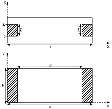
Fig. 1: A thick centered iris in a waveguide.

The thick centered iris in the waveguide shown in Fig. 1 can be analyzed by means of the equivalent circuit shown in Fig. 2, where the left and the right equivalent circuits refer to the discontinuities placed at Z=0 and Z=L, which can be considered as a transition between a regular rectangular waveguide of width a and a reduced waveguide of width d (and its opposite). The interconnecting lines represent the effects of the length L of the reduced waveguide.

post equivalent circuit

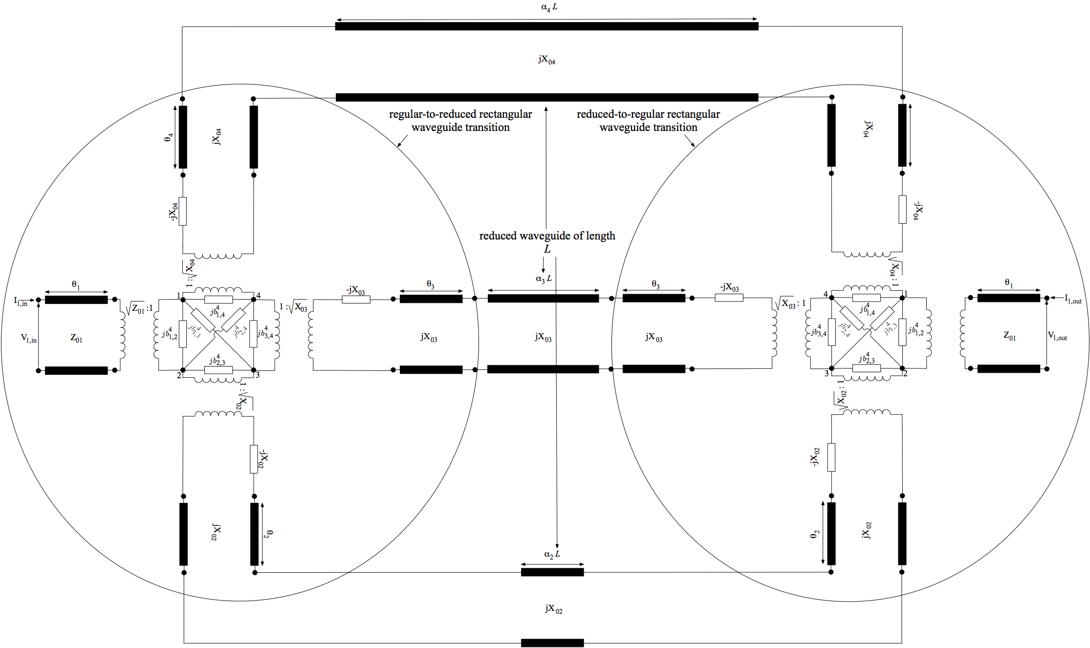
Fig. 2: The equivalent circuit for a thick centerd iris.

The left (or the symmetric right) circuit relative to the regular-to-reduced waveguide transition is shown in Fig. 3 in larger scale. If the reduced waveguide width is large enough, its fundamental mode becomes propagating and the equivalent circuit becomes the one shown in Fig. 4, where port #2 refers to the propagating output mode. Obviously, this equivalent circuit and the symmetric one replace the left and right ones in Fig. 2, if the fundamental mode in the reduced waveguide is above cutoff.

equivalent circuit

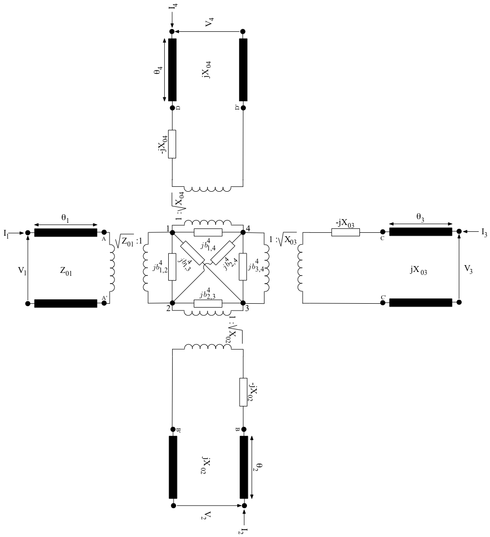
Fig. 3: The equivalent circuit for the regular-to-reduced waveguide transition placed at Z=0, if the fundamental mode of the reduced waveguide is below cutoff.

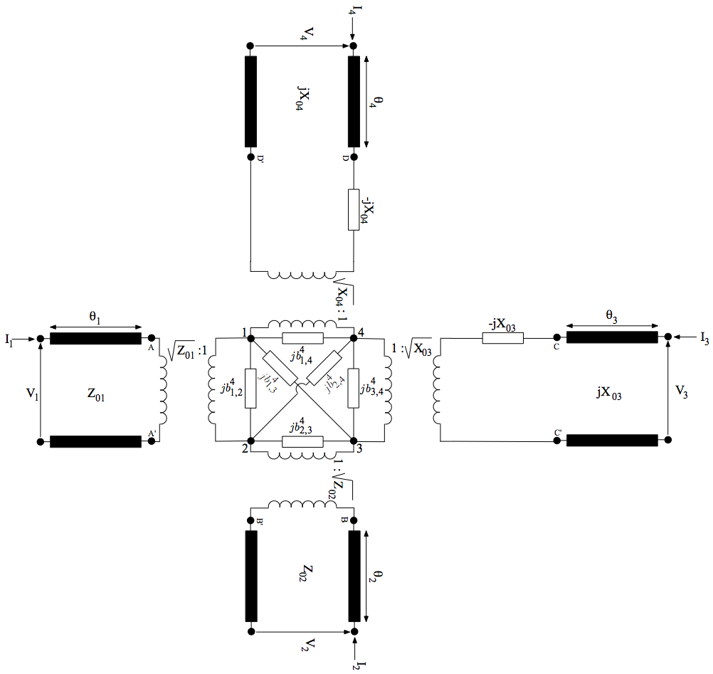
Fig. 4: The equivalent circuit for the regular-to-reduced waveguide transition placed at Z=0, if the fundamental mode of the reduced waveguide is above cutoff.

The susceptances $b_{i, j}^{4}$ and the electrical lengths $θ_{i}$ (i=1,2,3,4) in the equivalent circuit can be approximated with the following expansion (1), whose coefficients "c" are downloadable here for 1.25 < $\frac{f}{f_{c, 1}}$ < 1.9 , 0 < $\frac{w}{a}$ <1 and $n_{f}$ =12, $n_{w}$ =12, with $f_{c, 1}$ being the frequency cutoff of the fundamental mode of the regular waveguide of width a:

$\bar{ξ} = \sum_{k = 0}^{n_{f} - 1} \sum_{m = 0}^{n_{w} - 1} c_{k+1+m* n_{f}}^{ξ} {(\frac{f}{f_{c, 1}})}^{k} {(\frac{w}{a})}^{m}$ (1)

ξ= $b_{i, j}^{4}$ or $ξ {= θ}_{i}$

	0.1≤w/a≤0.2	0.2≤w/a≤0.3	0.3≤w/a≤0.4	0.4≤w/a≤0.5	0.5≤w/a≤0.526	0.526≤w/a≤0.54		0.54≤w/a≤0.56
Frequency range $\frac{f}{f_{c, 1}}$	1.25-1.9	1.25-1.9	1.25-1.9	1.25-1.9	1.25-1.9	1.25-a/w	a/w-1.9	1.25-a/w	a/w-1.9
Fundamental mode propagation: below (bc) or above (ac) cutoff	bc	bc	bc	bc	bc	bc	ac	bc	ac
$n_{f}$ , $n_{w}$	12,12	12,12	12,12	12,12	24,12	80,12	12,12	60,12	36,12
coefficients for (1) (xls format)	.xls	.xls	.xls	.xls	.xls	.xls	.xls	.xls	.xls
coefficients for (1) (txt format)	.txt	.txt	.txt	.txt	.txt	.txt	.txt	.txt	.txt

0.56≤w/a≤0.60

0.60≤w/a≤0.65

0.65≤w/a≤0.70

0.70≤w/a≤0.75

0.75≤w/a≤0.78

0.78≤w/a≤0.8

0.8≤w/a≤0.82

Frequency range

\frac{f}{f_{c, 1}}

1.25-a/w

a/w-1.9

1.25-a/w

a/w-1.9

1.25-a/w

a/w-1.9

1.25-a/w

a/w-1.9

1.25-a/w

a/w-1.9

1.25-a/w

a/w-1.9

1.25-1.9

Fundamental mode propagation: below (bc) or above (ac) cutoff

n_{f}

n_{w}

60,12

80,12

60,12

80,12

60,12

80,12

40,12

80,12

12,12

80,12

12,12

80,12

coefficients for (1) (xls format)

.xls

coefficients for (1) (txt format)

.txt

	0.82≤w/a≤0.85	0.85≤w/a≤0.90	0.90≤w/a≤0.95	0.95≤w/a≤0.99
Frequency range $\frac{f}{f_{c, 1}}$	1.25-1.9	1.25-1.9	1.25-1.9	1.25-1.9
Fundamental mode propagation: below (bc) or above (ac) cutoff	ac	ac	ac	ac
$n_{f}$ , $n_{w}$	24,12	12,12	12,12	12,12
coefficients for (1) (xls format)	.xls	.xls	.xls	.xls
coefficients for (1) (txt format)	.txt	.txt	.txt	.txt

The frequency cutoff of the fundamental mode of the reduced waveguide of width w is $f_{c, w} = \frac{c}{2 w}$ . The range of analysis of the transition is 1.25≤ $\frac{f}{f_{c, 1}}$ ≤1.9. Hence, by setting ${1.9 f}_{c, 1}$ = $f_{c, w}$ and ${1.25 f}_{c, 1}$ = $f_{c, w}$ , we can obtain the range of w/a where the fundamental mode of the reduced waveguide becomes propagating: 0.526≤w/a≤0.8. The second row of the tables follows this consideration by splitting the coefficient for (1) in the range below (bc) and above cutoff (ac).